Introduction
Consider the following scenario – you’ve just finished morning chores at your calf ranch and you’ve settled into the chair in front of the computer to enter some data and print a couple of reports. The phone rings. “Good morning! This is Sarah Bellim from Cheatham Feed Company. I’d like to tell you about our latest calf milk replacer supplement, Calf Explosion. Our latest research trial showed a statistically significant improvement in growth rates of calves that were fed Calf Explosion. Can I stop by tomorrow to tell you more about this exciting new product?” Hmmm, you think to yourself, statistically significant, eh? That sounds important. Maybe I should visit with Sarah about this new product…
But what does “statistically significant” really mean? And, what does it mean to you as a calf producer (or advisor)? This Calf Note is designed to address some of those questions.
Today, new technologies are being introduced every day. Improvements in nutrition, information, reproduction, health, and management occur at an ever increasing rate. When a producer incorporates these new technologies on the operation, a change is expected that will improve animal performance, lower cost of production or in some way improve economics of the operation.
But, we all know of new technologies (products and programs) that don’t work. There can be many reasons for the lack of an effect, but the fact remains, the product doesn’t work on your operation (or maybe it doesn’t work at all). So, how do you separate those products that are truly effective from those that are a waste of time and money? The first step is to understand the science behind the product. And, that’s where the term “statistically significant” comes in.
Variation – an example
Let’s look at what “statistically significant” means by way of a simple example. Say you have two groups of 100 calves. To the first group you feed a normal ration. We’ll call this group the “Control” group. To the second group you feed the normal ration plus feed additive “X”. You measure the body weight of the calves at the beginning and again at the end of the study.
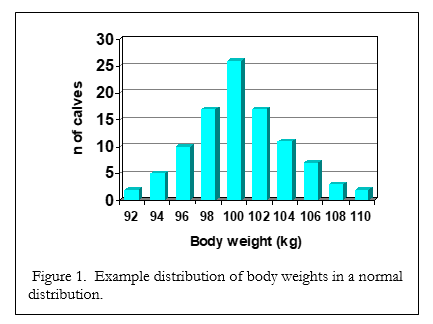
Let’s look at the control group first. All of these calves were fed the same diet, treated in the same way and so, they should all theoretically weigh the same at the end of the trial. Of course, not all calves weighed the same. Some calves grew faster than others due to their normal genetic makeup. Other calves consumed a little more milk replacer on some days than other calves. Still other calves developed diarrhea during the trial, which slowed their growth. If we take the average of the ending body weights of all the control calves, let’s say that average is 100 kg (220 lbs). But, there’s also variation associated with that average – i.e., some calves weighed more than the average (also called the mean) at the end of the study and some calves weighed less than the mean. For this example, let’s say that all the calves weighed between 92 and 110 kg at the end of the study. This variation around the mean can be calculated many different ways, but a common method is to calculate the standard deviation of the mean. Let’s say that the standard deviation of the mean for the control group was 4 kg. If we make a graph of the number of calves in each 2-kg category (say, 92-93.9 kg, 94-95.9 kg), we get a graph like figure 1. There is normal, random variation in the body weights and the distribution around the mean (100 kg) is called a “normal distribution”. This kind of distribution is also called a bell-shaped curve since it tends to look like a bell.
Now, let’s do the same with the calves fed the feed additive. The average ending body weight for this group of calves was 103.2 kg with a standard deviation of 5 kg.
We can use the two values (the mean and standard deviation) for each group to determine whether the difference between the two groups is really meaningful – i.e., is statistically significant. This is done using a specific series of procedures from statistics. Basically, these procedures compare the means from each treatment along with the variability around these means to determine whether the two means are the same (i.e., there was no effect of treatment “X”) or if the two means are different.
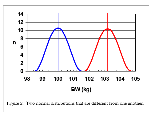
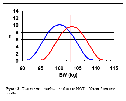
Look at Figure 2. We can quickly see that not only are the means different (the straight lines), but the variation around the means (the bell shaped lines) are also quite different. This is because there is no overlap between the two bell shaped curves. In Figure 3, we see that although the means are still the same (100 and 103 kg), there is much more variation around the means (i.e., the bell curves are much wider) and the distributions overlap one another. In this case, a statistical test would conclude that the means are NOT different from one another and treatment “X” did nothing in our test.
Two types of errors
When we do this types of testing, we make a conclusion based on the means and standard deviations of each group. We decide if the means are the same or are really different. And, of course, there’s a chance that our decision is wrong. In this case, there are two possible ways we could be wrong. The first kind of error (called type I error) occurs when we conclude that the means are different (there was a treatment effect) when there really wasn’t one. This is called a false positive – a good example is when a pregnancy test kit tells a woman that she’s pregnant when she really isn’t.
“Statistically significant”
By convention, most statistical tests control the risk of false positives by saying that we want to be correct 95% of the time when we conclude that the treatment means are different. This also means that we’ll be wrong (i.e., we conclude that there was a difference between treatments when one didn’t exist) only 5% of the time. This is where “P < 0.05” comes from. The probability of making the wrong conclusion is 5% or less.
So, when someone says the two means are different at P < 0.05, it means that if the experiment were repeated 100 times under the same conditions, then 95% of the time the results would be similar to the first experiment. While the mean values might not be exactly the same, the relative differences should be similar.
It has been tradition that the term “statistically significant” or “significant” means P < 0.05. However, some researchers may consider statistically significant to be P < 0.10 instead of P < 0.05. Generally, it’s easier to show “significance” when you use a higher P value. It’s important that you understand what someone means when they say “significant”. The important question is “if it’s significant, at what level of probability – 5%, 10% or another level?”
What does this mean to you?
People throw around the term “statistically significant” with great abandon these days. However, there are some important implication and cautions that you as a consumer of the information should be aware of. Here are some points to consider when looking at the results of research trials:
- The goal of most researchers is to find a statistically significant difference if one exists. This means that it’s important for him or her to reduce the variation in the experiment as much as possible (e.g., trying to get graphs like Figure 2 instead of Figure 3). To accomplish this, researchers control as many aspects of the research as possible – animals, diets, management, housing, environment, etc. This control increases the ability of a researcher to see a difference, but what effect does this have on you? The variability on your operation may be greater because you can’t control all the variables like a researcher. This is the most common reason that producers try new products but can’t see the differences promised by the proponents of the new technology.
- Under what conditions was the research conducted? Researchers may artificially control the conditions of the experiment to increase the chance to get a statistical difference. It may be possible to see an improvement in growth from birth to weaning when a feed additive is added to milk replacer fed at 454 g/d without feeding added calf starter; however, how many producers actually don’t feed starter to their calves during the first eight weeks of life? Look for artificial management in the research, which should set off alarm bells about the true viability of the technology.
- Be careful about populations. Often calf researchers work with bull calves (esp. preweaning) because bull calves are cheaper to purchase and use in research. We usually make the assumption that data collected with bull calves will be applicable to heifer calves. But, is this always true? Be aware if the researchers use breeds other than the one you use on your operation, also.
- Beware small studies! The rules of statistics say that if you have a small number of experimental animals, it’s harder to declare statistical significance. However, a small number of animals may also mean that the animals are much more uniform, thereby reducing variability. This may make the results of the research less applicable in the “real world”. I generally like to see a minimum of 25-30 calves per treatment in research with young calves. I view results from studies that use 10 calves or less with caution.
- What is the magnitude of the difference between treatments in research? Many researchers get excited about statistical significance but lose sight of the actual numbers. It might be possible to see a significant difference of 250 grams of body weight gain per day – what does this mean to a producer? Even under the best conditions, you’ll never be able to measure a 250 gram increase in daily gain on the farm.
- What’s the P value being used?
- What’s being measured? Many calf researchers measure parameters such as body weight gain, height gain, feed efficiency, etc. Are you measuring these parameters on your operation? Are they important to you – if your calves are 5 kg heavier at weaning, what does this mean to you from an economic standpoint? Consider the measurements in question and how the change may affect your operation.
- What is the value proposition? If you invest $1 per calf per day in a new technology, what do you expect to get back? What is the ROI (return on investment) – the economic benefit divided by cost. For example, you invest $10,000 per year in a technology that reduces death loss of preweaned calves by 5%, which saves you $50,000 per year. The ROI is 50,000 / 10,000 = 5:1. Most producers look for a minimum ROI of 3:1.